Introduction to ggpaintr

Introduction

Grammar of Graphics & ggplot2

First proposed by (Wilkinson, Anand, and Grossman 2005), the grammar of graphics defines a way of concisely breaking up graphs into semantic components for data visualization. Analogous to the grammar in English, the grammar of graphics tells us which “words” should be used to make up a “sentence”. It allows users to create a complex graphic by assembling multiple independent components.

The open-sourced R package ggplot2 (Hadley Wickham 2010) implemented this grammar of graphics with some modifications and refinements, leading to what is now called a ‘’layered grammar’’. ggplot2 built a mapping from the data to geometric objects in multiple different layers drawn on a coordinate system. As an example, the code following this layered grammar to complete a line chart can include:

• A base layer with raw data;

• A layer for drawing the lines;

• A layer for specifying x, y labels and the title;

• A layer for legend settings;

• A layer for choosing background theme;

• …

Each of the above functionalities can be modularized into one or several functions. Modules are assembled together at high level of abstraction according to the “grammar” of ggplot2, to eventually show the graphic we desire.

Compared to the plotting functions in vanilla R, ggplot2 is more convenient to use, with higher flexibility and readability. It is considered one of the most popular R package (H. Wickham 2016).

Building a Shiny App with Graphical Visualization

Shiny is a framework for creating web applications from R. Shiny apps built from R shiny help users interact with the data instead of facing the ice-cold coding console. Together with ggplot2, it provides possibility of creating elegant data visualizations with large flexibility. Interactive graphical visualizations are extremely helpful in presentations or statistical education (Doi et al. 2016), for providing the audience with a clear and straight forward view of data analysis.

However, the procedure of building such a fancy shiny app may not be as fancy as it comes out. It requires an extensive knowledge about shiny and comes at a cost of heavy and tedious programming work:

• The implementation of each component in the grammar of graphics requires an unignorable amount of coding;
• Some functionalities in ggplot2 may not be able to realized easily and intuitively in shiny (e.g., the customization of colors);
• Most importantly, apart from the code for individual ggplot components, there’s a lot of extra work to do for assembling them into a real shiny app.

Our Contribution

In this manuscript we introduce our package ggpaintr, a package for building shiny apps with ggplot2 visualizations. Using our package, the programming work for building a data-visualization shiny app can be dramatically reduced, while the coding structure is rather simplified and mimics the way ggplot2 works in R.

Why ggpaintr can be useful

The goal of ggpaintr is to make it easy for writing shiny apps. ggpaintr is a collection of highly modularized shiny app components. It offers the possibility to build a shiny app for ggplot2 data visualization with minimum effort. The resulting shiny app can achieve broader functionality than the ggplot GUI, while the code to accomplish this is much more readable and logical.

Our package has the following advantages:

1. Simplicity

   Not only is the code using ggpaintr much shorter, it is also much more readable comparing to using vanilla shiny functions.

2. Flexibility

   We have implemented ready-to-use modules in ggpaintr for most of the commonly used ggplot2 arguments. By calling those modules directly users can achieve almost any complex functionality they desire. As an example, a shiny app built from our pacakge can achieve the following visualization:

   ggplot(data) + 
     geom_point(aes(x, y, color, fill), size, alpha) + 
     facet_grid(z ~ w) + 
     coord_flip() + 
     labs(x = ..., y = ..., title = ...) + 
     theme(...) + 
     ...

3. Extensibility

   Moreover, if you are familiar with shiny and want to extend the functionality to something we haven’t implemented, our package also offers the ability (and instructions) of providing your own ui and server functions, and even adding new modules into the package (?).

ggpaintr is a user-friendly package. Anyone with some knowledge of ggplot2 can start building a shiny app with basic ggplot output like the one shown below, after a self-teaching of ggpaintr for less than 10 minutes:

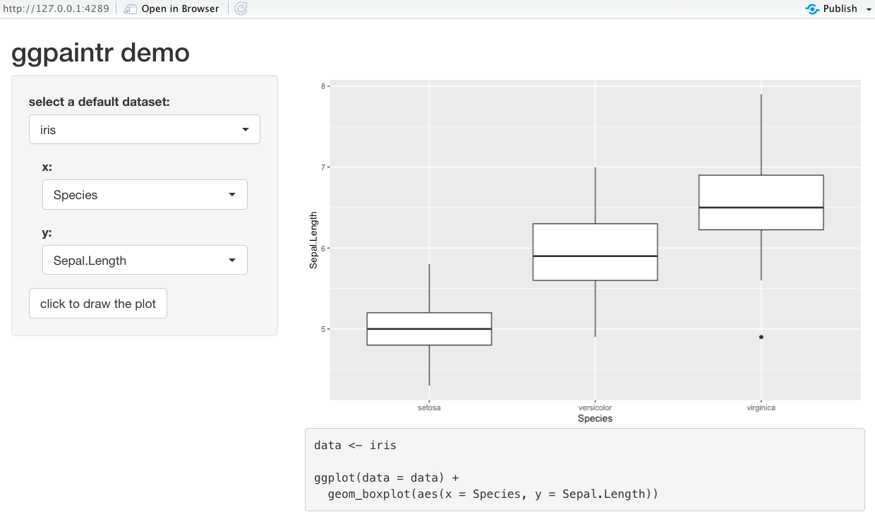
Sample Iris Shiny App

And more complex options and functionalities can be added and achieved using similar logic within a few lines of code. Currently ggpaintr has implemented most of the commonly used ggplot2 functions and their parameter options. You will learn in details about how to implement them in the next section.

We expect this package to be useful in the following scenarios:

• Statistical education of graphics

  Our package offers a easier and more flexible way of building graphical shiny apps. Statistics instructors can develop interactive graphical UIs on their own with their specific demands. By transforming R’s programming language into a point-and-click style, these UIs can be used to introduce different statistical graphics to fresh students in this field.

• Statistical education of R / ggplot2

  Along with the plot, shiny apps built from our package also interactively show the complete R code for generating such plot. This can be extremely useful for beginners in R or ggplot2.

• Graphical demos in presentation

  The most important characteristic of ggpaintr is that users can customize their app based on their demand and preference. We have implemented modules for most of the commonly used functionalities in ggplot2, and the grammar used in ggpaintr is also similar. As long as you are familiar with ggplot2, you should not find it hard to build your own shiny app. With some extra knowledge of shiny, you also have the ability to convert it into a fancier style as a formal presentation demo.

Installation

You can install the development version from Github with:

# install.packages("devtools")
devtools::install_github("willju-wangqian/ggpaintr")

Case Study 1: ggpaintr demo

Let’s revisit the demo shiny app presented in Figure X. After selecting a dataset, the shiny app allows users to map variables (or columns) in the dataset to x and y. It generates a plot using ggplot2 and shows the corresponding R code. The reactivity on the mappings are built up so that changing mappings variables for x or y will change the resulting plot after clicking the “draw” button. Moreover, changing the selected dataset will automatically update the available choices for x and y. Without the help of ggpaintr, building such a shiny app at least requires the following steps:

• have UI components for x and y so that input$x and input$y are available
• dynamically render UI components for x and y so that the available choices depend on the selected data set
• figure out how to generate a ggplot2 plot using input$x and input$y since the inputs are strings. One option is to use aes_string()
• figure out the R code for generating the resulting plot
• render the plot
• render the code

This might look involved, but what if this shiny app needs more functionalities? If the shiny app needs more mappings, such as color or fill, it will add more UI component, modify the server part so that the inputs can be correctly captured. If the shiny app wants to allow users to flip the coordinates using coord_flip() or adding labels using labs(), building this shiny app becomes even more involved. Additionally, maintaining and updating the shiny app can be challenging as well since many aspects of the shiny app would be modified.

However, we can build such a shiny app using ggpaintr with the following code.

library(ggpaintr)
library(shiny)
library(tidyverse)
library(shinyWidgets)
library(palmerpenguins)

# Define UI for application that draws a histogram
ui <- fluidPage(
  
  # Application title
  titlePanel("ggpaintr demo"),
  
  # Sidebar with a slider input for number of bins
  sidebarLayout(
    sidebarPanel(
      pickerInput("defaultData", "select a default dataset:",
                  choices = c("iris", "mtcars","penguins", "faithfuld"),
                  selected = "",
                  multiple = TRUE,
                  options = pickerOptions(maxOptions = 1)),
      uiOutput("controlPanel"),
      actionButton("draw", "click to draw the plot"),
    ),
    
    # Show a plot of the generated distribution
    mainPanel(
      plotOutput("outputPlot"),
      verbatimTextOutput('outputCode')
    )
  )
)

# Define server logic required to draw a histogram
server <- function(input, output) {
  
  control_id <- "control_id"
  
  # data
  data_container <- reactive({
    req(input$defaultData)
    get(input$defaultData)
  })
  
  # construct paintr object
  paintr_rctv <- reactive({
    
    req(data_container())
    
    paintr(control_id,
           data_container(), data_path = input$defaultData,
           geom_boxplot(aes(x, y)) 
    )
    
  })
  
  # place ui
  output$controlPanel <- renderUI({
    req(paintr_rctv())
    
    column(
      12,
      paintr_get_ui(paintr_rctv(), "x"),
      paintr_get_ui(paintr_rctv(), "y"),
    )
  })
  
  # take results and plot
  observe({
    req(paintr_rctv(), data_container(), input$defaultData)
    data <- data_container()
    
    paintr_results <- paintr_plot_code(paintr_rctv())
    
    # Plot output
    output$outputPlot <- renderPlot({
      
      paintr_results[['plot']]
      
    })
    
    # Code output
    output$outputCode <- renderText({
      
      paintr_results[['code']]
      
    })
    
  }) %>% bindEvent(input$draw)
  
  
}

# Run the application
shinyApp(ui = ui, server = server)

Many things are hidden and handled by functions in ggpaintr, and we will talk about it in detail in the next section. Updating this shiny app can be relatively easy with the help of ggpaintr: by changing the ggplot2 alike expression at line 51 into

# add mapping for fill
geom_boxplot(aes(x, y, fill)) +
  coord_flip +        # allow users to flip coordinate
  labs(x, y, title)   # allow users to add labels for x-axis, y-axis, and title

and adding more elements in output$controlPanel <- renderUI() at line 57:

# place ui
output$controlPanel <- renderUI({
  req(paintr_rctv())
  
  column(
    12,
    paintr_get_ui(paintr_rctv(), "x"),
    paintr_get_ui(paintr_rctv(), "y"),
    paintr_get_ui(paintr_rctv(), "fill"),
    paintr_get_ui(paintr_rctv(), "coord_flip"), # add UI for coord_flip()
    paintr_get_ui(paintr_rctv(), "labs"),       # add UI for labs()
  )
})

we can build a shiny app with the updated features as shown in Figure X. We can see that the shiny app now allows users to flip coordinates and set labels. The plot and corresponding R code can be updated accordingly as well.

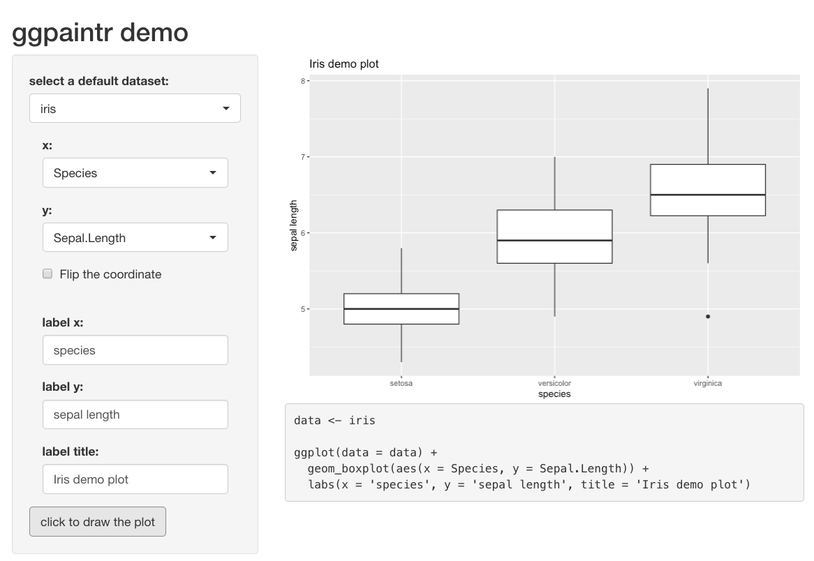
An Extended Iris Shiny App

ggpaintr Design Desicisions

Basic Structure

Making a shiny app with ggpaintr is straightforward. Since the UI components of mapping (and other plot settings like coord_flip() or labs()) are dynamically rendered, we will need a uiOutput(id) on the UI side that serves as a placeholder for the dynamically rendered UIs, like line 21 in the code of the demo shiny app. Another thing needed on the UI side is an action button, which is closely related to the design on the server side. On the server side, there are three building blocks that we need to take care of:

• creating a paintr_obj object using ggpaintr::paintr() as a reactive value (line 45).

  paintr(
    id,
    data,
    expr,
    extra_ui = NULL,
    extra_ui_args = NULL,
    data_path = "data"
  )

  paintr() is the main function of ggpaintr and returns a paintr_obj object. It expects three arguments:

  • id: this ID will be used to create a namespace shared by all UI and module servers related to this paintr_obj object.
  • data: the dataset used to generate the plot
  • expr: an expression that controls which functionality should be included in the shiny app.

  Note that wrapping the paintr_obj with reactive() is not required by the paintr() function, but required by the reactivity in the shiny app. Therefore, one can create a paintr_obj using paintr() and inspect its structure and elements even outside the context of a shiny app:

  my_paintr <- paintr("id", iris, 
                      geom_boxplot(aes(x, y, fill)))

• extract the UI element using ggpaintr::paintr_get_ui() (line 62).

  paintr_get_ui(
    paintr_obj,
    selected_ui_name,
    type = "ui",
    scope = NULL,
    verbose = FALSE
  )

  paintr_get_ui() expects a paintr_obj object and a selected key name for the ui. This selected key name can be any key name that has been implemented in ggpaintr or a user-defined key name. This will be discussed later in detail. paintr_get_ui() returns the UI element of the selected key name and returns NULL if the selected key name is not included in the expr of paintr(). paintr_get_ui() can be used to obtain the ID of the selected UI element if type = "id". This is useful since the ID of the UI element of a selected key name can potentially be arbitrary if the UI function is user-defined.

• generate the plot and corresponding R code using paintr_plot_code() (line 72)

  paintr_plot_code(
    paintr_obj,
    selected_color_rctv = NULL,
    selected_fill_rctv = NULL,
    color_fill = FALSE,
    color_group = FALSE,
    userFUN = NULL,
    ...
  )

  paintr_plot_code() takes a paintr_obj object and executes all of the module server functions in order to generate the resulting plot using ggplot2 and the corresponding R code. Note that paintr_plot_code() is designed to be wrapped by observeEvent(), or equivalently by the combination of observe and bindEvent introduced by Shiny 1.6.0. The isolate() environment provided by observeEvent() can prevent the module server functions from execution when necessary pieces are missing. As a result, an action button that controls paintr_plot_code() and observeEvent() is expected on the UI side.

Control with Expressions

The expression expr in paintr() is essential to the functionality of ggpaintr. It controls what type of plot the shiny app can make and what functionalities the shiny app provides. In general, a valid expr is as the following:

geom_<chart>(aes(<mapping_1>, <mapping_2>, ...), <geom_args_1>, <geom_args_2>, ...) +
  <plot_settings_1> +
  <plot_settings_2> + 
  ...

• geom_<chart> can be any geom_ functions in ggplot2 as long as the required aesthetic mappings are correctly provided.
• <mapping_*> are the key names for the aesthetic mapping. Currently, we have implemented x, y, z, fill, color, shape, size, and group. These are the most commonly used aesthetic mappings and will allow users of the shiny app to select variables from the dataset for a specific mapping. The UI elements of these mapping key names are implemented with shinyWidgets::pickerInput(), which allow users to select and deselect.
• <geom_args_*> are the key names for arguments passed into the geom_<chart> function. Currently, we have implemented alpha, size, position, and stat. The UI elements of size and alpha accept numeric inputs, and the UI elements of position and stat are shinyWidgets::pickerInput(), which provides a list of options for the users. We are able to use strings to control position and stat but have not included all the string options. Since position, stat, and other arguments of a geom_<chart> can be very complicated in ggplot2. We plan to have a more sophisticated way of handling the arguments in the future.
• <plot_settings_*> are the key names for functions that can modify the plot in higher layers. Currently, we have implemented coord_flip, facet_grid, theme_choose, scale_color, scale_fill, theme(legend.position, legend.direction, legend.box), and labs(x, y, title, subtitle). Note that theme_choose allows users of the shiny app to choose themes from a list (theme_gray(), theme_classic(), theme_bw(), theme_minimal()) and is not a function in ggplot2. This shows that both the key names and the ui and server part associated with the key name can be customized. Another thing worth noting is that theme() in ggplot2 is very powerful but we only have implementations for three of its parameters: legend.position, legend.direction, and legend.box. We were able to implement these three parameters because they require strings instead of ggplot2::element_*. labs(x, y, title, subtitle) is similar to theme(). And currently, labs can only set labels for x, y, title, and subtitle. scale_color and scale_fill will be discussed later.

Modularity

The idea of modularized shiny app largely inspired our design of ggpaintr. Each key name, no matter it is <mapping>, <geom_args>, or <plot_settings>, can be considered as a module. It can have its own ui and server functions and is independent of other key names’ modules. Once the key name is included in the expr of paintr(), its ui function will be executed when paintr() is called, and its server function will be executed when paintr_plot_code() is called. Modularization allows us to implement different modules independently and provides the possibility for other developers to include their own modules. It also provides the flexibility in building shiny apps using ggpaintr. At the same time, maintaining and updating certain features of a shiny app become easier since we only need to work on the module that is responsible for the change.

Flexibility in UI Design

Developers who build shiny apps using ggpaintr have a lot of freedom in their design of the user interface. The UI element of a key name can be obtained by paintr_get_ui(), and a developer has full control on how or where to put it in the shiny app. If the default UI element of a key name does not meet the need of a developer, one can provide their own ui functions and override the default.

Reactivity

scale_color and scale_fill allow users of the shiny app to manually select colors for color and fill, respectively. Since color and fill have similar behaviors, we will use color for further explanation. If a numerical variable is mapped to color, scale_color_gradient() is used, and users can select one color for low and another color for high; if a categorical variable is mapped to color, scale_color_manual() is used, and the colors selected by the users are passed into the parameter values of scale_color_manual(). If the categorical variable has more than 11 levels, the server function for scale_color will refuse to render the ui for choosing colors and give a warning message.

The ui for choosing colors are implemented with colourpicker::colourInput and depends on the selected variable of color or fill mapping. That is, the reactivity between scale_color and color requires the existence of color and some user input, and thus it cannot be established at the same time when the reactive value of paintr() is created. To solve this problem, we implemented a function called scaleColor_build_reactivity(), which can establish the reactivity for both color and fill.

scaleColor_build_reactivity(
  id, 
  paintr_obj, 
  color_or_fill
)

• id should be the same id used for paintr(). This ensures that the modules share the same name space.
• paintr_obj is a reactive value of a paintr_obj object created by paintr()
• color_or_fill specifies color or fill

In order to add reactivity for fill in our demo shiny app, one should make the following changes:

• change the expression expr to include scale_fill and establish the reactivity:

  paintr_rctv <- reactive({
  
      req(data_container())
  
      paintr(control_id,
             data_container(), data_path = input$defaultData,
             geom_boxplot(aes(x, y, fill)) +
                 coord_flip +
                 labs(x, y, title) +
                 scale_fill
      )
  })
  
  scale_fill_rctv <- scaleColor_build_reactivity(control_id, paintr_rctv, "fill")

• modify the ui output:

  output$controlPanel <- renderUI({
      req(paintr_rctv())
  
      column(
          12,
          paintr_get_ui(paintr_rctv(), "x"),
          paintr_get_ui(paintr_rctv(), "y"),
          paintr_get_ui(paintr_rctv(), "fill"),
          paintr_get_ui(paintr_rctv(), "coord_flip"),
          paintr_get_ui(paintr_rctv(), "labs"),
          paintr_get_ui(paintr_rctv(), "scale_fill") # added for scale_fill
      )
  })

• pass the reactive object scale_fill_rctv into paintr_plot_code()

  paintr_results <- paintr_plot_code(paintr_rctv(),
                                     selected_fill_rctv = scale_fill_rctv)

Extensibility

This part needs some future work.

Case Study 2: ggpaintr_app

A shiny app called ggpaintr_app is built with the ggpaintr package and included in the package. ggpaintr_app not only demonstrates the functionality of ggpaintr, but also serves as a shiny app for those unfamiliar with the Grammar of Graphics or ggplot2 but want to create a plot using ggplot2. Some design of ggpaintr_app can also provide reference for package/shiny app developers.

Run the shiny app

library(ggpaintr)

run_ggpaintr_app()

Home page

Our Home page gives a brief introduction about the ggpaintr package and the corresponding shiny app,it also includes our GitHub repository link, which can direct users to our package codes if needed.

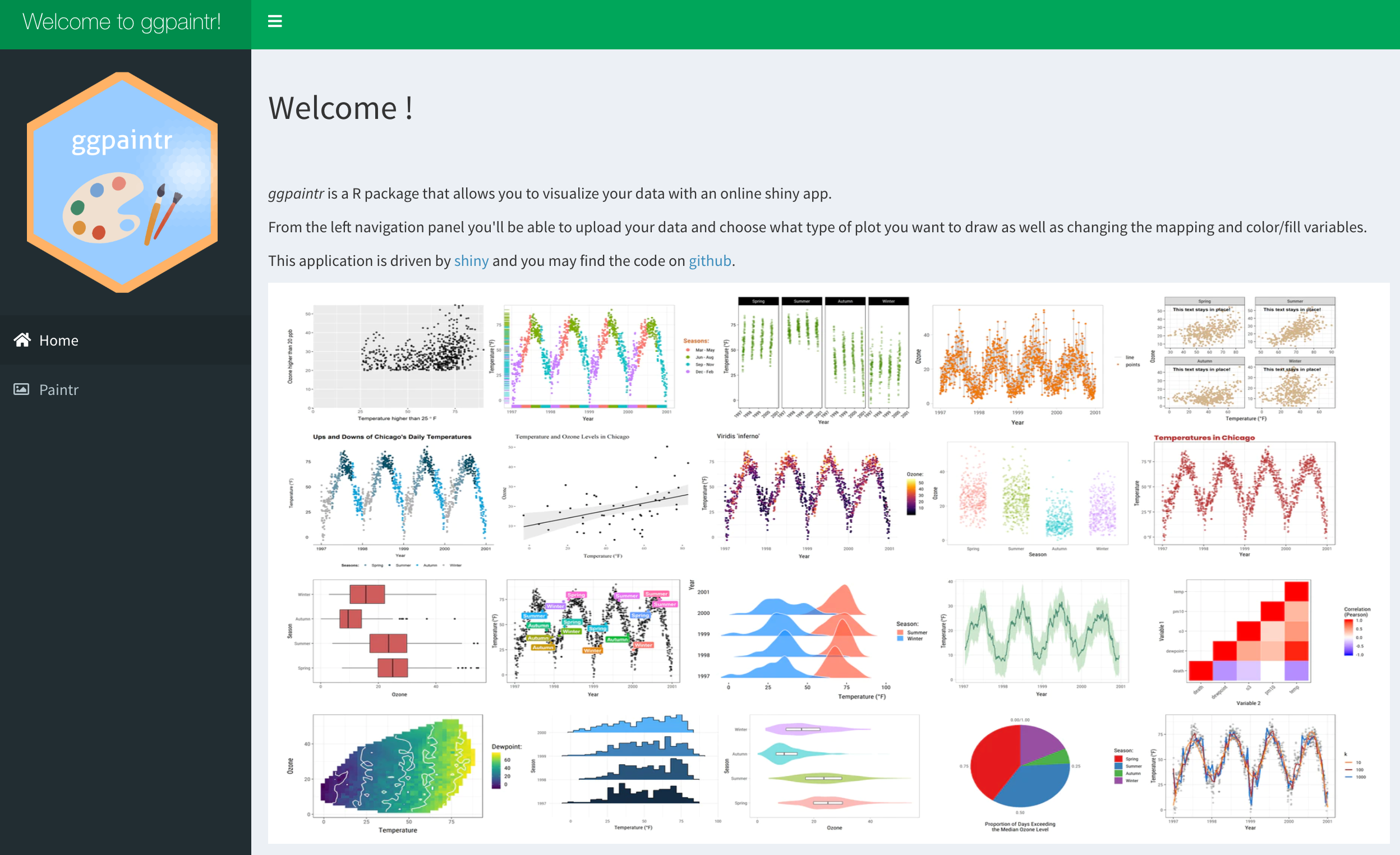
Homepage.

Paintr page

The Paintr page is the main user interface of the app, this page is further divided into three tabs, which are Data, Paint, and Code.

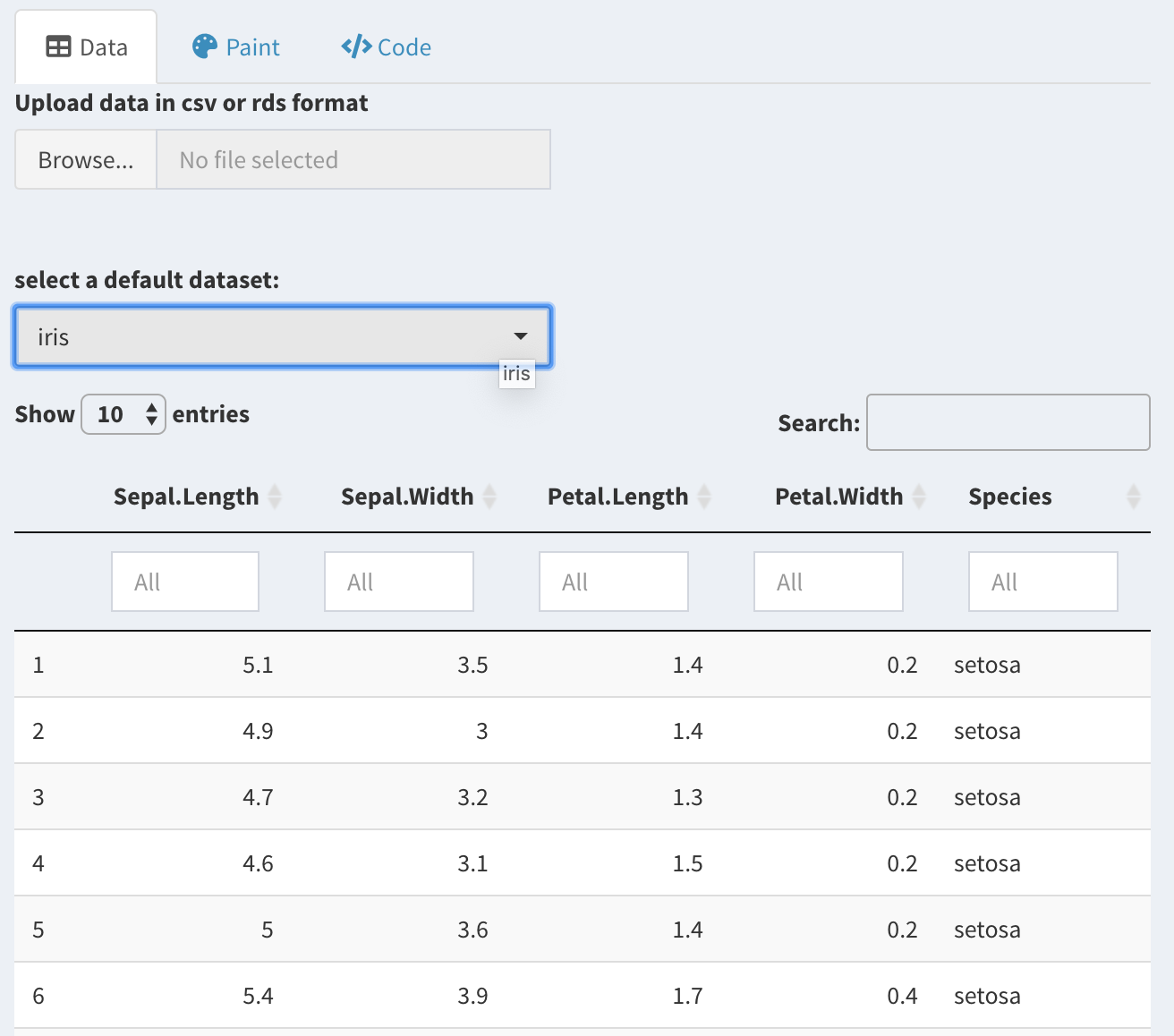
1.Data tab

Under Data, users are allowed to either upload data set from their local file folders, or select a data set from Base R database.

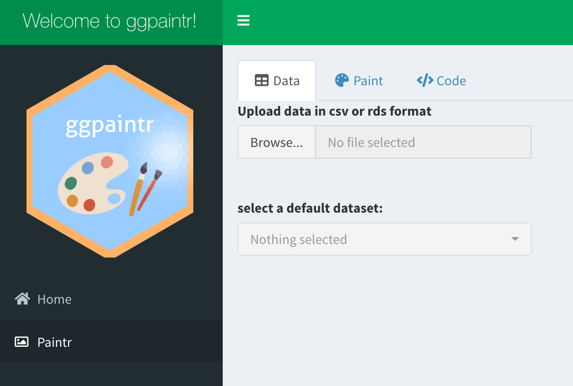
Paintr page.

Once the data set is loaded, users can see partial example of the data set and even filter the data before moving to the next step.

Filter function.

2.Paint tab

Under Paint, there are image icons to present all types of plots currently available in our shiny app, these image icons allow users to choose the type of plot they would like to draw in a more intuitive manner.

Once the type of plot is chosen, the corresponding mapping options box will pop up. Here, we have embedded basic mapping options such as x, y, color, fill, and size; we also included advanced setting where users can modify the legend,coordinate, theme, labels or facet the plot.

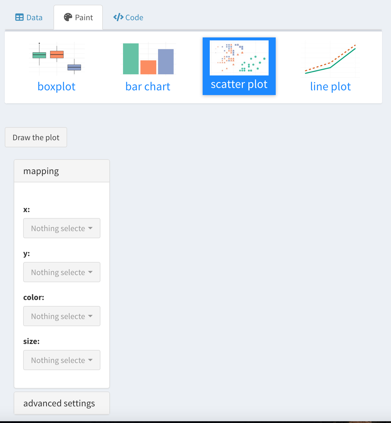
Paint page.

What’s more, in order to meet different aesthetic needs, it also allows users to freely choose colors for their plots.

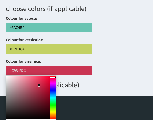
Paint page.

Once all the mapping variables and setting options are chosen, users can click the Draw the plot button and the plot will show up automatically. Here is an example of a scatter plot drew with the iris data.

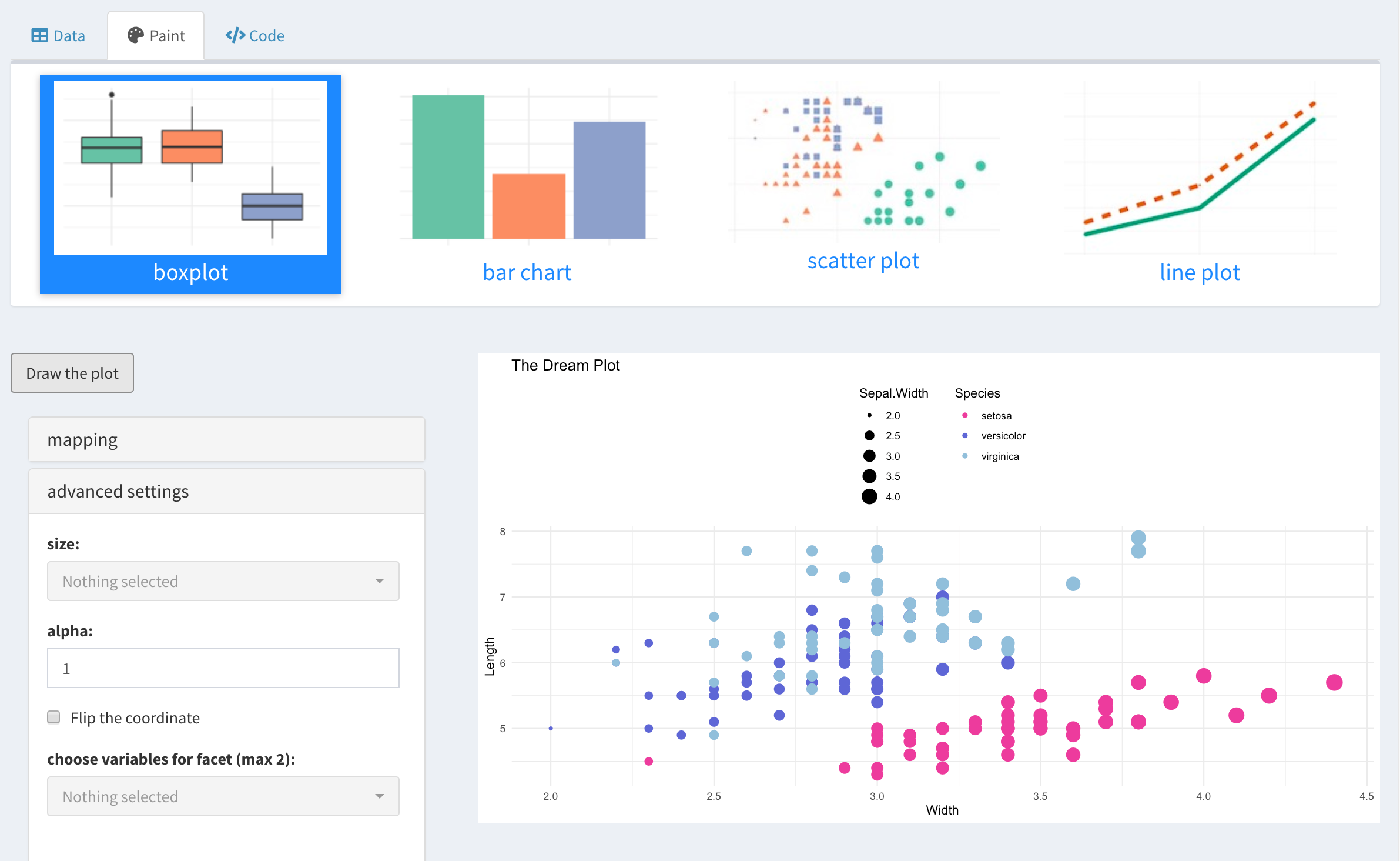
Example plot.

3.Code tab

Although we have included most of the mapping and aesthetic options for drawing a plot in our shiny app, we want to give users more freedom to modify their plots if needed. Therefore, the code for drawing the plot will also be provided once a plot is made. Simply copy and paste the code into R console and run it will generate an identical plot as the shiny app does. Modify the codes and draw your dream plot is also encouraged.

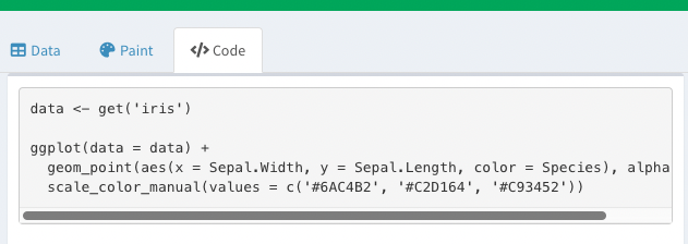
Example code.

Conclusion

In this project, we introduced an open-source R package ggpaintr for building modularized shiny apps with plotting functionalities using ggplot2 and the idea of the Grammar of Graphics. We showcased what ggpaintr can do with two case studies in this project and discussed the thoughts and decisions we had in the designs of ggpaintr. We combined the idea of modularization and the Grammar of Graphics and implemented independent modules that are responsible for different pieces of the plotting functionality of a shiny app. ggpaintr makes it easier to embed reactive plotting functionality in a shiny app and provides simplicity, flexibility, and extensibility. With the help of ggpaintr, reactive plotting in a shiny app can be easily achieved and updated since an expression in ggplot2-alike syntax can control which modules or reactivity to be included in the shiny app. So far, we only implemented the most commonly used and basic features of ggplot2. However, as an open-source R package, developers can easily develop their own modules, cover more aspects of ggplot2, and make suggestions and improvements for ggpaintr. We aim to build a bridge between ggplot2 and shiny apps, connecting versatility and interactivity. We hope that ggpaintr can make it easier for statistics researchers and educators to build interactive data visualizations, lower the bar on learning ggplot2 while keeping its elegance and flexibility, and in turn encourage more students to step into this field.

References

Doi, Jimmy A., Gail E. Potter, Jimmy Wong, Irvin Alcaraz, and Peter Chi. 2016. “Web Application Teaching Tools for Statistics Using r and Shiny.” Technology Innovations in Statistics Education 9.

Wickham, H. 2016. Ggplot2: Elegant Graphics for Data Analysis. Use r! Springer International Publishing. https://books.google.com/books?id=RTMFswEACAAJ.

Wickham, Hadley. 2010. “A Layered Grammar of Graphics.” Journal of Computational and Graphical Statistics 19 (1): 3–28. https://doi.org/10.1198/jcgs.2009.07098.

Wilkinson, Lee, Anushka Anand, and Raymond Harold Grossman. 2005. “Graph-Theoretic Scagnostics.” IEEE Symposium on Information Visualization, 2005. INFOVIS 2005., 157–64.