ptr_app(
  ggplot(mtcars, aes(x = ppVar, y = ppVar)) + geom_point()
)2 Getting Started
ggpaintr turns a ggplot2 call into a Shiny app. You write the plot the way you always do, drop a placeholder keyword wherever a reader of your app should get to choose a value, and hand the whole expression to ptr_app(). Each placeholder becomes an input widget; clicking Update plot re-runs the call with the user’s choices spliced back in.
This chapter takes you from zero to a running app, then to an app that boots with sensible defaults. Code in this book is shown verbatim and not executed; the running UI is shown as a screenshot captured from a tested fixture (see the welcome page for how that stays honest).
2.1 Your first app
The smallest useful app is one line. ppVar marks a spot where the user picks a column:
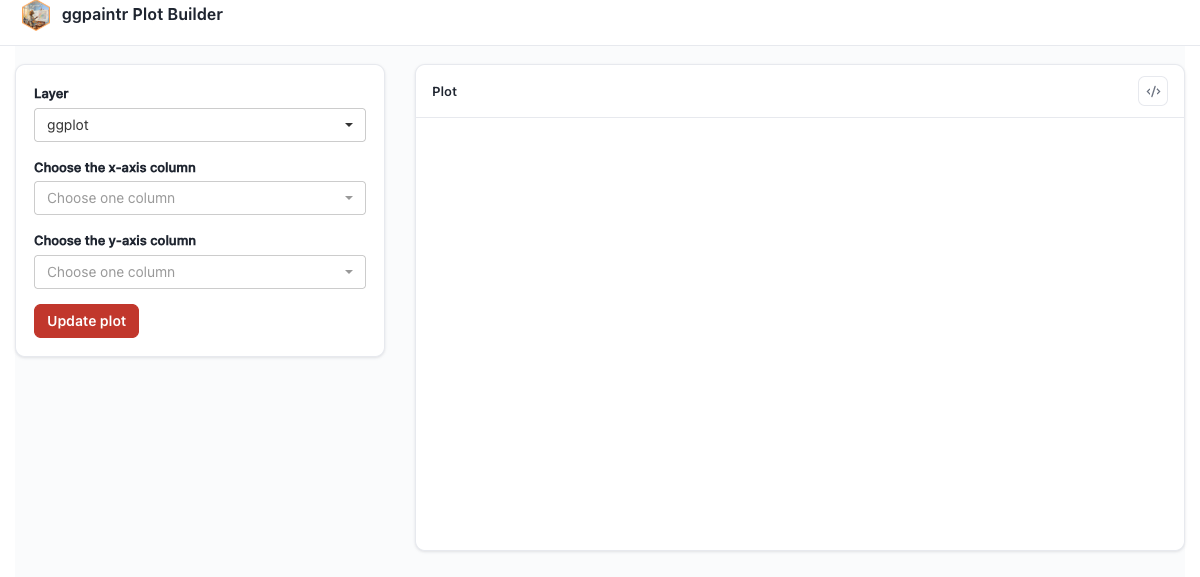
ppVar, and the Update plot button. The plot pane stays empty until the first update.Three things are worth noticing before you click anything:
- There is no
data =argument toptr_app(). The bare symbolmtcarsis resolved in your calling environment, exactly as it would be if you ran theggplot()call directly. The only required argument is the formula itself. - The dropdowns already know the columns.
ppVaris data-aware: it lists the columns of whatever data flows into it. - Nothing renders yet. By default, ggpaintr re-draws only when Update plot is clicked. Changing a widget stages a value; the button commits it. This keeps a half-typed input from strobing the plot.
Pick wt and mpg, click Update plot, and the scatterplot appears — along with the generated ggplot2 code behind the </> toggle, ready to copy back into a script (Chapter 5).
2.2 Seeding the widgets
An app that boots with empty pickers makes the user do all the work. Give any placeholder a single positional argument and it becomes the widget’s starting value:
ptr_app(
  ggplot(mtcars, aes(x = ppVar("wt"), y = ppVar("mpg"))) +
    geom_point(size = ppNum(3), alpha = ppNum(0.6)) +
    labs(title = ppText("Weight vs. mileage"))
)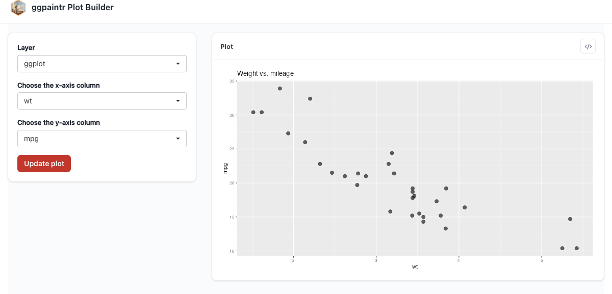
wt and mpg are pre-picked, the size and alpha inputs start at 3 and 0.6, and the title is pre-filled.The seed is read literally from the formula text — it is never evaluated as user code. (ppNum does accept simple arithmetic like ppNum(2 * pi), folded at build time against a small allowlist; see Chapter 3.)
2.3 The chrome you get for free
Every app built with ptr_app() ships the same furniture, all driven by the formula with no configuration:
ptr_app(
"ggplot(mpg, aes(displ, hwy)) +
geom_point(alpha = ppNum(0.5)) +
geom_smooth(method = ppText('loess'))"
)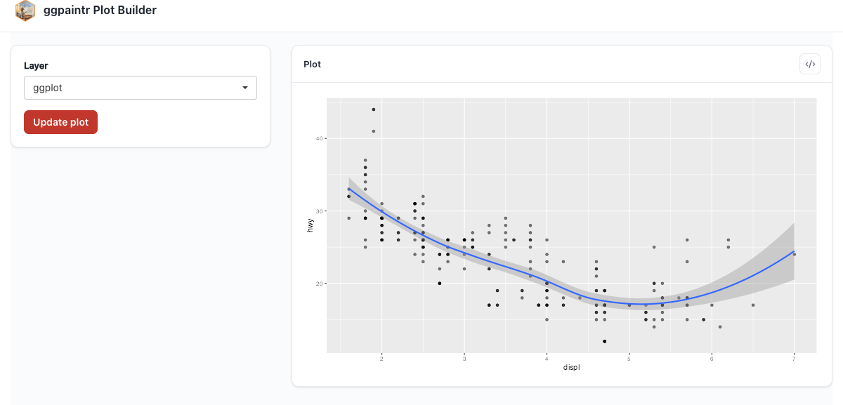
ggplot, geom_point, and geom_smooth; each layer shows only its own placeholders.- The layer picker. One entry per layer in the formula; selecting a layer shows that layer’s widgets. Layers carrying no placeholder still appear, so the user sees the whole chart’s structure.
- The Data subtab. When a layer’s data argument is a pipeline (Chapter 4), its stages get widgets and per-stage toggles here.
- The code window. The
</>toggle opens the generated code — Final code and Spec views, with a Copy button (Chapter 5). - The Update plot button. Nothing redraws until it is clicked (Chapter 3).
(The string formula above works exactly like the bare-code form used so far — both are covered in Chapter 4.)
2.4 Using your own data
ppVar placeholders need syntactic, unique column names — Sepal.Length is fine, "Sepal Length" is not, and iris deliberately ships clean. If your local data has spaces, reserved words, or duplicates in its names, pipe it through ptr_normalize_column_names() before referencing it from a formula:
messy <- data.frame(
  check.names = FALSE,
  "first column" = 1:3,
  "if"           = 4:6
)
clean <- ptr_normalize_column_names(messy)

ptr_app("ggplot(clean, aes(x = ppVar('first_column'), y = ppVar('if_'))) + geom_point()")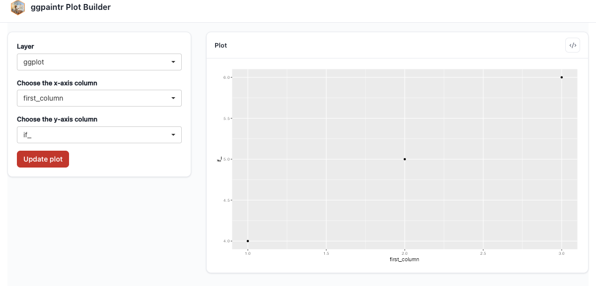
first column became first_column, the reserved if became if_.Uploaded data is normalized automatically; the manual call is only for data already in your session. The exact rules are in Chapter 5 and ?ptr_normalize_column_names.
2.5 Where to go next
- Chapter 3 introduces all five built-in placeholders and the three roles they play.
- Chapter 4 covers the formula as a language: pipelines ahead of
ggplot(), and boot-state toggles likeppLayerOff. - Chapter 5 explains the code panel and how empty inputs clean themselves out of the generated code.
- Chapter 6 shows how to register widget types of your own — most real apps end up wanting at least one.
- Chapter 20 (the book’s final part) is a collection of complete, realistic examples — each one paired with the plain ggplot2 plot it parameterizes.